|
Home
APS
Downloads
Buy APS
Support
Register
Contact us
Knowledge Base of APS
Subscribe to the GEPList
Visit GEP
|
|
The APS Environment
|
|
| Evolving a Model |
| |
In order to evolve a model with APS 3.0 you must first choose the problem category which is chosen while you are loading the input data for modeling. There are three different types of problem category in APS 3.0:
Function Finding, Classification, and Time Series
Prediction, each using a specific learning algorithm and requiring special features.
To Evolve a Model with Automatic Problem Solver 3.0
- In the Settings Panel, select the General Settings Tab and then choose the appropriate settings for your problem.
For all types of problems, the most important is the chromosome architecture, that is, the number of genes, the head size and the linking function.
- In the Functions Panel, choose the appropriate set of functions to model your data.
Automatic Problem Solver 3.0 offers a great variety of built-in functions (a total of 70 functions). Besides, APS 3.0 also allows you to create both static and dynamic user-defined functions and evolve complex models with them.
Static UDFs allow you to establish a permanent relationship between specific independent variables, for instance UDF1 = do + d1 + d2 + d3, and use this new UDF as an extra terminal in your modeling kit.
Dynamic UDFs are much more powerful and interesting than static UDFs as they behave exactly like the built-in functions of APS and therefore can be used to model all kinds of relationships between variables or complex expressions. For instance, you can design DDF1 so that it will model the sum of four variables or expressions, that is, DDF1 = (expression 1) + (expression 2) + (expression 3) + (expression 4), where the value of each expression will depend on the context of DDF1 in the expression tree. A note of caution, though, although extremely interesting, DDFs decrease the speed of the algorithm somewhat and therefore we advise you to choose your functions from the wide set of APS 3.0 built-in functions.
- In the Settings Panel, select the Fitness Function Tab and choose the fitness function.
Automatic Problem Solver 3.0 provides you with 11 built-in fitness functions for
Function Finding and
Time Series Prediction problems and
10 different fitness functions for Classification problems. In addition, APS 3.0 also allows you to create your own fitness functions and therefore allows you to explore even more solution
landscapes.
- In the Settings Panel, select the Genetic Operators Tab and choose the appropriate degree of genetic variation.
Automatic Problem Solver 3.0 offers several genetic operators which allow you to introduce the ideal degree of genetic modification in order to allow an efficient evolution of your models. If you are overwhelmed by all these operators, please use the defaults as they work very well for all problems.
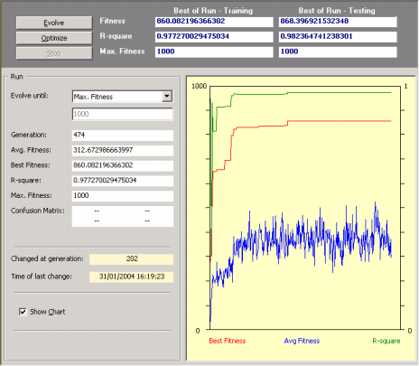
- In the Run Panel, click the Evolve button.
Automatic Problem Solver 3.0 shows all the essential parameters of the best-of-generation model during the discovery process. Whenever you are satisfied with the result, just press the Stop button. Your best-of-run model is ready either for analysis or scoring. And if you are still not happy with the results, you can still try to fine-tune the evolved model by pressing the Optimize button.
|
|
| Home | Contents |
Previous | Next
|
|