So, for time series prediction, the art of good modeling consists basically in finding ways around this strong attractor. And the learning algorithms of APS 3.0 provide you with the necessary tools and strategies for finding good time series predictive models. The most important are outlined below:

• Choose a well balanced function set so that the discovery of a model of only one argument (obviously, the t-1 variable) does not come easily. For instance, if you are using an embedding dimension of 12 and your function set consists of only the four arithmetical operators, you must weight proportionately the representation of each function in the function set, otherwise the creation of complex models will be seriously compromised. A good rule of thumb is to use at least as many functions in the function set as there are independent variables, which, in time series prediction, corresponds exactly to the embedding dimension.
• Start the modeling process with a relatively complex architecture, say, 4-5 genes with a head size of 6-8, in order to make it difficult for the algorithm to stumble upon this strong attractor.
• Or you can start with a simpler architecture, say, one gene with a head size of 6-8, but then stop the evolutionary process before the attractor is found (or you can stop the evolutionary process when the attractor is found, as APS 3.0 allows you to select any of the best-of-generation models of a run and use it as seed). Then you can use one of these models to genetically modify the seed by introducing an additional neutral gene. This neutral gene paves the way to more complex models. Theoretically, by repeating this process, you can approximate any continuous function to an arbitrary precision if there is a sufficient number of terms.
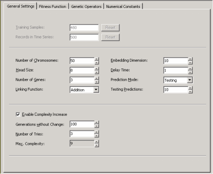
• APS 3.0 also allows you to increase the complexity of your model automatically by activating the Complexity Increase Engine in the Settings Panel -> General Settings Tab. Then you must fill the Generations Without Change box to choose the period of time you think acceptable for evolution to occur without improvement in best fitness, after which a mass extinction or a neutral gene (an extra term) is automatically added to the evolving models; the Number of Tries box corresponds to the number of consecutive evolutionary epochs (defined by the parameter Generations Without Change) you will allow before a neutral gene is introduced in all evolving models; in the Max. Complexity box you write the maximum number of terms (genes) you’ll allow in your model and no other terms will be introduced beyond this threshold.

So, the evolutionary strategies we recommend in the APS templates for Time Series Prediction are all oriented toward the creation of models with good predictive power. This means that the models created using the templates will be highly sophisticated and will require a considerable amount of time to design. However, if you whish to create less complex models you can stop the evolutionary process any time you see fit and check its capabilities at making predictions about the future in the Predictions Panel. Then you can try to design a better model by continuing the evolutionary process with your current model as seed.

APS 3.0 chooses the appropriate template for your problem according to the number of variables in your data. This kind of template is a good starting point that allows you to start the modeling process immediately with just a mouse click. Indeed, even if you are not familiar with evolutionary computation in general and gene expression programming in particular, you will be able to design complex nonlinear models immediately thanks to the templates of APS 3.0. In the provided templates, all the adjustable parameters of the learning algorithm are already set and, for instance, you don’t have to know how to create genetic diversity, how to set the appropriate population size, the chromosome architecture, the fitness function, how to increase the complexity of your models, and so forth. Then, as you learn more about APS, you will be able to explore all its modeling tools and create quickly and efficiently very good models that will allow you to make accurate predictions about the future.

There is, however, a very important setting in APS that is not controlled by APS 3.0 templates and must be wisely chosen by you: the number of Training Samples which, in time series prediction, depends not only on the size of the time series but also on the Embedding Dimension, the Delay Time, and the Prediction Mode.

Thus, in practice, the embedding dimension corresponds to the number of independent variables or terminals after your time series has been transformed and, therefore, will have a strong impact on the complexity of the problem. The delay time t determines how data are processed, that is, continuously if t = 1 or at t intervals.

As stated for Function Finding or Classification problems, the larger the training set the slower evolution or, in other words, the more time will be needed for generations to go by. So, you must compromise here and choose a training set with the appropriate size. A good rule of thumb consists of choosing 8-10 training samples for each independent variable in your data.

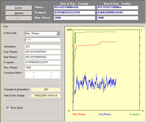
So, after creating a new run you just have to click the Evolve button in the Run Panel in order to design a model. Then you observe carefully the evolutionary process, especially the plot for best fitness. Then, whenever you see fit, you can stop the run without fear of stopping the evolutionary process prematurely as APS 3.0 allows you to continue the evolutionary process at a later time by using the best-of-run model as the starting point (evolve with seed). For that you just have to click on the Optimize button in the Run Panel.

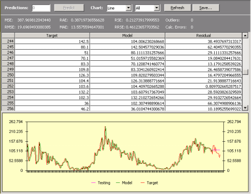
This strategy has enormous advantages as you might choose to stop the run at any time and then take a closer look at the evolved model. For instance, you can analyze its mathematical representation, evaluate its performance in the testing predictions, check a wide set of statistical functions for a quick and rigorous assessment of its accuracy, make a few predictions with it, and so on. Then you might choose to adjust a few parameters, say, choose a different fitness function, expand the function set, add a neutral gene, and so forth, and then explore this new evolutionary path. You can repeat this process for as long as you want or until you are completely satisfied with the evolved model.

In addition, if you wish for APS 3.0 to increase the complexity of your models automatically, you just have to activate the Complexity Increase Engine and then click the Evolve button and APS will evolve better and better models composed of an increasing number of terms until no increase in best fitness takes place for a certain period of time.