Automatic Problem Solver 3.0 offers a total of 70 built-in mathematical
functions, including 24 IF THEN ELSE rules, that can be used for designing nonlinear regression models. This wide set of mathematical functions allows the evolution of complex and rigorous models quickly built with the most appropriate functions.
Despite the wide set of APS built-in mathematical functions, some users sometimes want to model with different ones. APS 3.0 gives the user the possibility of creating custom tailored functions
(dynamic UDFs or DDFs) and evolve models with them. A note of warning though: the use
DDFs slows considerably the evolutionary process and therefore should be used with moderation.
Below are listed all the 70 built-in functions available in APS 3.0, including their representation in
Karva (given in brackets) and their mathematical definition:
Basic mathematical functions of two arguments:
- Addition (+): x+y
- Subtraction (-): x-y
- Multiplication (*): x*y
- Division (/): x/y
- Floating-point Remainder (Mod): mod(x,y)
- Power (Pow): pow(x,y)
Basic mathematical functions of one argument:
- Square Root (Sqrt): sqrt(x)
- ex (Exp): exp(x)
- 10x (Pow10): pow(10,x)
- Natural Logarithm (Ln): ln(x)
- Logarithm Base 10 (Log): log(x)
- Logistic (Logi): logistic(x)
- Floor (Floor): floor(x)
- Ceiling (Ceil): ceil(x)
- Absolute Value (Abs): abs(x)
- Inverse (Inv): 1/x
- No Operation (Nop): x
- Negation (Neg): -x
Trigonometric functions (x is in radians):
- Sine (Sin): sin(x)
- Cosine (Cos): cos(x)
- Tangent (Tan): tan(x)
- Cosecant (Csc): csc(x)
- Secant (Sec): sec(x)
- Cotangent (Cot): cot(x)
Inverse trigonometric functions:
- Arcsine (Asin): arcsin(x)
- Arccosine (Acos): arccos(x)
- Arctangent (Atan): arctan(x)
- Arccosecant (Acsc): arccsc(x)
- Arcsecant (Asec): arcsec(x)
- Arccotangent (Acot): arccot(x)
Hyperbolic functions:
- Hyperbolic Sine (Sinh): sinh(x)
- Hyperbolic Cosine (Cosh): cosh(x)
- Hyperbolic Tangent (Tanh): tanh(x)
- Hyperbolic Cosecant (Csch): csch(x)
- Hyperbolic Secant (Sech): sech(x)
- Hyperbolic Cotangent (Coth): coth(x)
Inverse hyperbolic functions:
- Inverse Hyperbolic Sine (Asinh): arcsinh(x)
- Inverse Hyperbolic Cosine (Acosh): arccosh(x)
- Inverse Hyperbolic Tangent (Atanh): arctanh(x)
- Inverse Hyperbolic Cosecant (Acsch): arccsch(x)
- Inverse Hyperbolic Secant (Asech): arcsech(x)
- Inverse Hyperbolic Cotangent (Acoth): arccoth(x)
Comparison 0/1 functions of two arguments:
- OR1 (OR1): if x < 0 OR y < 0, then 1; else 0
- OR2 (OR2): if x >= 0 OR y >= 0, then 1; else 0
- AND1 (AND1): if x < 0 AND y < 0, then 1; else 0
- AND2 (AND2): if x >= 0 AND y >= 0, then 1; else 0
Comparison IF THEN ELSE functions of two arguments (series A):
- If Less Than (IFA1): if x < y, then x; else
y
- If Greater Than (IFA2): if x > y, then x; else
y
- If Less Than Or Equal To (IFA3): if x <= y, then
x; else y
- If Greater Than Or Equal To (IFA4): if x >= y, then
x; else y
- If Equal To (IFA5): if x = y, then x; else
y
- If Not Equal To (IFA6): if x != y, then x; else
y
Comparison 0/1 IF THEN ELSE functions of two arguments (series B):
- If Less Than (IFB1): if x < y, then 1; else 0
- If Greater Than (IFB2): if x > y, then 1; else 0
- If Less Than Or Equal To (IFB3): if x <= y, then 1; else 0
- If Greater Than Or Equal To (IFB4): if x >= y, then 1; else 0
- If Equal To (IFB5): if x = y, then 1; else 0
- If Not Equal To (IFB6): if x != y, then 1; else 0
Comparison IF THEN ELSE functions of three arguments (series C):
- If Less Than (IFC1): if x < 0, then y; else z
- If Greater Than (IFC2): if x > 0, then y; else z
- If Less Than Or Equal To (IFC3): if x <= 0, then y; else
z
- If Greater Than Or Equal To (IFC4): if x >= 0, then y; else
z
- If Equal To (IFC5): if x = 0, then y; else z
- If Not Equal To (IFC6): if x != 0, then y; else z
Comparison IF THEN ELSE functions of four arguments (series D):
- If Less Than (IFD1): if a < b, then c; else
d
- If Greater Than (IFD2): if a > b, then c; else
d
- If Less Than Or Equal To (IFD3): if a <= b, then
c; else d
- If Greater Than Or Equal To (IFD4): if a >= b, then
c; else d
- If Equal To (IFD5): if a = b, then c; else
d
- If Not Equal To (IFD6): if a != b, then c; else
d
By selecting the Functions (Math) Tab in the Functions
Panel, you have full access to the 70 built-in mathematical functions of APS 3.0. Here is also the place where you can add
Dynamic UDFs (DDFs) to your modeling kit.
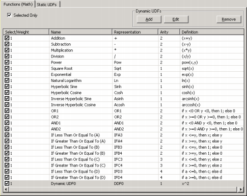
To select a function, just check the box on the left. By default, the weight of each function is 1, but you can increase the probability of a function being included in your models by increasing its weight in the Select/Weight column. The weight property is very important for a successful modeling, as the overall number of functions used in a run must be well balanced with the number of terminals or variables in your data. For instance, if you are modeling data with hundreds of variables and using only the four arithmetical operators, you must weight proportionately the representation of each function in the function set, otherwise the creation of complex models will be seriously compromised. A good rule of
thumb is to have at least as many functions in the function set as there are variables.
To add a DDF to your modeling kit, just click the Add button on the Dynamic UDFs frame and the DDF editor appears.
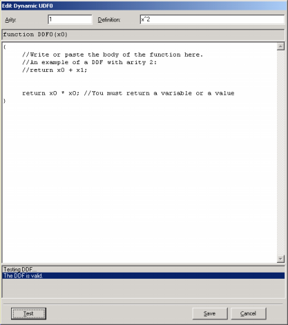
By choosing the arity (minimum is 1 and maximum is 4) in the Arity box, the function header appears
in the code window. Then you just have to write the body of the function in the code editor. The code must be in JavaScript and can be
conveniently tested for compiling errors.
In the Definition box, you can write a brief description of the function for your future reference. The text you write here will appear in the Definition column.
Dynamic UDFs are extremely powerful and interesting tools as they are treated exactly like the built-in functions of APS and therefore can be used to model all kinds of relationships between variables or complex expressions. For instance, you can design a DDF so that it will model the sum of four expressions, that is, DDF = (expression 1) + (expression 2) + (expression 3) + (expression 4), where the value of each expression will depend on the context of the DDF in the expression tree. A note of caution, though, although extremely interesting, DDFs decrease considerably the speed of the algorithm and therefore we advise you to choose your functions from the wide set of APS 3.0 built-in functions.
|