The successful creation of Time Series Prediction models requires the use of very sharp modeling tools. The most important are listed below.
Time Series Transforming Engine
Before modeling, the data in a time series must be transformed so that it can be used to create prediction models.
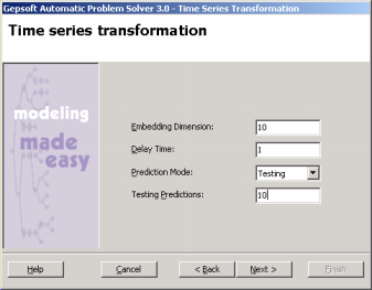
Automatic Problem Solver 3.0 comes with a time series transforming engine that transforms the time series according, obviously, to the
Embedding Dimension and Delay Time, but it also transforms the time series depending on whether you wish to make predictions about the future or test the predictive power of the evolved models on known past behavior.
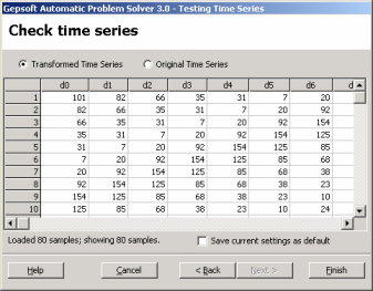
You can then observe the transformation on the Testing Time Series window before proceeding with the new
run.
The time series transforming engine of APS 3.0 is operational every time you create a new run or every time you change either the
Embedding Dimension or the Delay Time, the Prediction Mode or the
number of Testing Predictions during a
run in the General Settings Tab.
In practice, the embedding dimension corresponds to the number of independent variables (terminals) after your time series has been transformed. The delay time
t determines how data are processed, that is, continuously if
t = 1 or at t intervals.
These two parameters, together with the size of the time series and
the prediction mode, will determine the final number of training samples after the transformation of the time series.
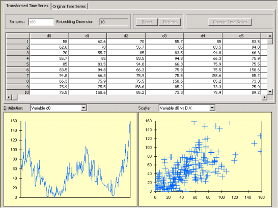
The data are then ready for evolving prediction models with them and can be visualized in the Data
Panel before evolving a new model.
Data Screening Engine
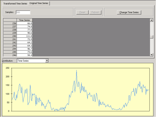
Time series have a simple data format which consists of a column of time series observations.
Automatic Problem Solver 3.0 data screening engine makes sure that the right format is fed into the time series transforming engine of APS 3.0 so that the time series is transformed correctly either to create a model for making predictions or testing the predictive potential of the model against known behavior.
Data Visualization Tool
The data visualization tool of APS 3.0 enables you to analyze the distribution of all the inputs.
The visualization of the distribution of all data points is a valuable modeling tool as it can help you detect outliers in your data that can then be removed so that better models are created. Typographical or measurement errors generally cause outliers that can be detected by analyzing the time series graphically.
Built-in Fitness Functions
Automatic Problem Solver 3.0 offers a total of 11 built-in fitness functions based on well-known statistical functions.
Fitness functions are fundamental modeling tools for they determine the nature of the search landscape. And different fitness functions open and explore different paths in the solution space. The fitness functions of APS 3.0 are named as follows:
Relative with SR,
Relative/Hits, Absolute with
SR, Absolute/Hits,
R-square, MSE,
RMSE, MAE,
RSE, RRSE, and
RAE.
User Defined Fitness Functions
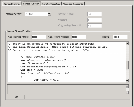
Despite the wide set of APS built-in fitness functions, some users sometimes want to experiment with fitness functions of their own. Automatic Problem Solver 3.0 gives the user the possibility of creating custom tailored fitness functions and evolve models with them.
The code for the custom fitness function must be in JavaScript and is written in the Custom Fitness Function window and can be tested before evolving a model with it.
Built-in Mathematical Functions
Automatic Problem Solver 3.0 offers a total of 70 built-in mathematical
functions. This wide set of mathematical functions allows the evolution of complex and rigorous models quickly built with the most appropriate functions.
From the simple arithmetic operators to complex mathematical functions available in most programming languages to more complex mathematical functions commonly used by engineers and scientists, the modeling algorithms of APS 3.0 enable you the integration of the most appropriate functions in your models.
Dynamic User Defined Functions (DDFs)
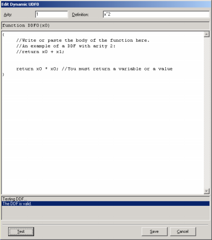
Despite the wide set of APS built-in mathematical
functions, some users sometimes want to model with different ones. APS 3.0 gives the user the possibility of creating custom tailored functions and evolve models with them. A note of warning though: the use of dynamic UDFs slows considerably the evolutionary process and therefore should be used with moderation.
The code for the DDFs must be in JavaScript and is written in the Edit DDF window (in the Functions Panel, select the Functions (Math) Tab and then click Add in the Dynamic UDFs tool box).
Static User Defined Functions (UDFs)
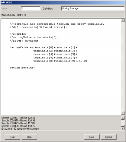
Sometimes it is possible to spot relatively simple relationships between certain variables in your data, and APS 3.0 allows you to use this information to build custom tailored functions
(UDFs). These functions allow the discovery of more complex models composed of several simpler models.
The code for the UDFs must be in JavaScript and is written in the Edit UDF window (in the Functions Panel, select the Static UDFs Tab and then click Add in the Static UDFs tool box).
Learning Algorithms
Automatic Problem Solver 3.0 is equipped with two different algorithms for evolving complex nonlinear prediction models.
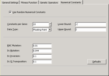
The first is the fastest and simplest of the two. And because it is also the most efficient, this algorithm is the default in APS 3.0. The second algorithm is very similar to the first, with the difference that it gives the user the possibility of choosing the range and type of numerical constants that will be used during the learning process.
In order to evolve models using the second algorithm, select Numerical Constants in the Settings Panel and then check the box that activates this algorithm. You will notice that additional parameters become available, including a small set of genetic operators especially developed for handling numerical constants (if you are not familiar with these operators, please use the default values for they work very well in all cases).
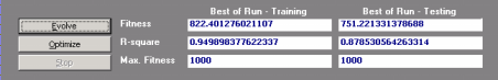
Monitoring the Modeling Process
Automatic Problem Solver 3.0 allows you to monitor the modeling
process by plotting the essential parameters of a run during the discovery process, including average fitness and the fitness and R-square of the best-of-generation model.
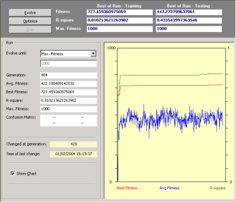
The evolutionary process can be stopped whenever you are satisfied with the results by pressing the Stop button or you can use one of the stop criteria of APS for picking up your model exactly as you want it.
When the evolutionary process stops, the best-of-run model is ready either for analysis or scoring. And if you are still not happy with the results, you can still try to fine-tune the evolved model by pressing the Optimize button and repeat this process until you are completely satisfied with your model.
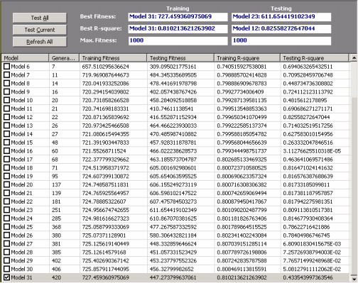
Analyzing Intermediate Models
Automatic Problem Solver 3.0 gives you the possibility of gaining some insights into the modeling process by analyzing all the best-of-generation intermediate models.
All the best-of-generation models discovered during a run are saved and you can pick them up for analysis at the
History Panel by checking the model you are interested in. Each of these intermediate models can then be analyzed exactly as you do for the best-of-run model, that is, you can check their performance in the testing set, check their vital statistics, automatically generate code with them, visualize their parse trees, use them as seed to create better models from them and so forth.
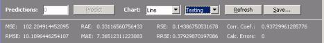
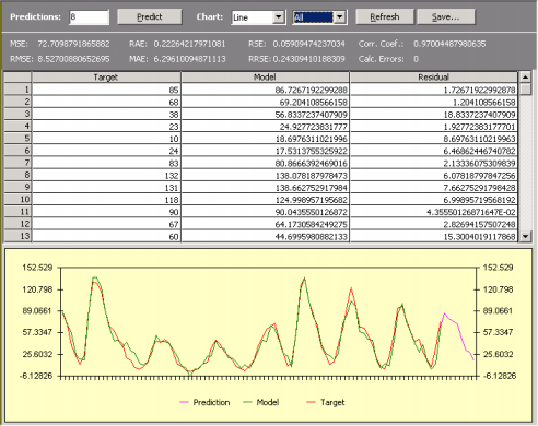
Comparing Actual and Predicted Values
Automatic Problem Solver 3.0 offers two different ways of analyzing and comparing the output of your model with the actual or target values both for training and testing.
In the first, the target or actual values are listed in a table side by side with the predicted values.
In the second, the target and predicted values are plotted in a chart for easy visualization.
And both table and chart are shown simultaneously in the Predictions
Panel.
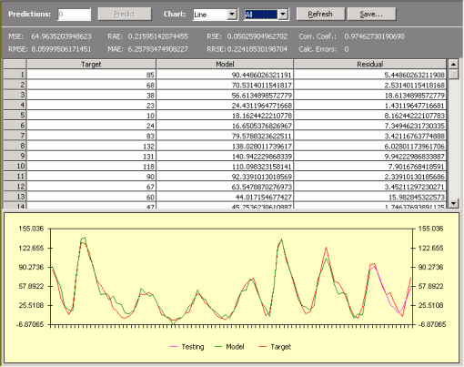
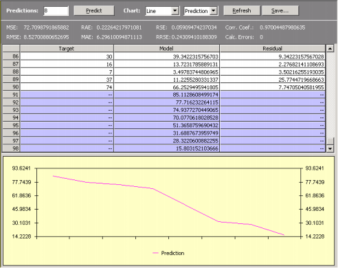
If you are testing the predictive power of your model using past known observations, the comparison of the predictions with the actual values are listed at the end of the table highlighted in
blue and are also plotted in the chart. In addition,
these testing predictions can either be observed together with the
training results or separately in a different plot.
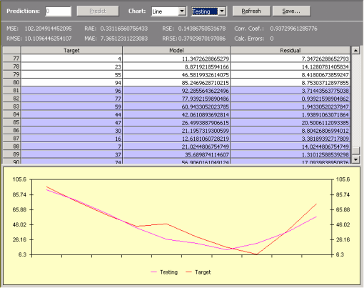
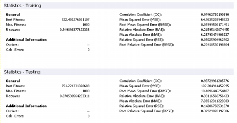
Essential Statistics
Automatic Problem Solver 3.0 allows a quick and easy assessment of a wide set of
statistical
functions. Most of them are immediately computed and shown every time you check the Results Panel
(for instance, mean squared error,
root mean squared error,
mean absolute error,
relative squared error,
root relative squared
error, relative absolute
error, R-square,
and correlation
coefficient).
If you are testing the predictive power of your model using past known observations, you can also check the same set of statistical indexes
(mean squared error,
root mean squared error,
mean absolute error,
relative squared error,
root relative squared
error, relative absolute
error, and correlation
coefficient)
obtained for the recursive testing, by selecting Testing in the
Chart options. You’ll notice that the values of the statistical functions
are updated, and they refer to the results obtained in the testing.
These and other statistical functions (R-square, correlation
coefficient and fitness)
are also shown in the Report Panel so that they can be used for future reference, but you must check them first in the
Predictions Panel.
Modeling from Seed
Automatic Problem Solver 3.0 allows the use of an existing model (which could have been either generated by APS or by another modeling tool) as the starting point of an evolutionary process so that more complex, finely tuned models could be created.
For models created outside of APS 3.0 or for APS 3.0 models modified by the user, the starting model or seed is fed to the algorithm through the Change Seed window where both the fitness and structural soundness of the model are tested.
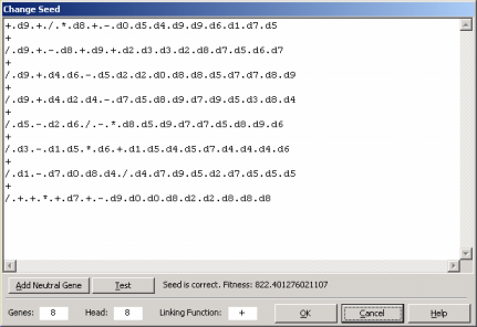
Then, in the Run Panel, by clicking the Optimize button, an evolutionary process starts in which all the subsequent models will be descendants of the seed you introduced. A note of caution though: if your seed has a very small fitness, you risk loosing it early in the run as better models could be randomly created by APS 3.0 and your seed, most probably,
would not be selected for breeding new models. If your seed has zero fitness, though, you will receive a warning so that you could modify your seed until it becomes a viable seed capable of breeding new models.
For models created in the APS 3.0 environment, the seed is fed to the algorithm every time you click the Optimize button during modeling, with the seed (in this case, the best model of the previous run) being introduced automatically by
APS.
Adding a Neutral Gene
The addition of a neutral gene to a seed might seem, at first sight, the wrong thing to do as most of the times we are interested in creating efficient and parsimonious models. But one should look at this as modeling in progress as, for really complex phenomena, it is not uncommon to approximate a complex function progressively.
Thus, being able of introducing extra terms to your seed is a powerful modeling tool and APS 3.0 allows you to do that through the Change Seed window.
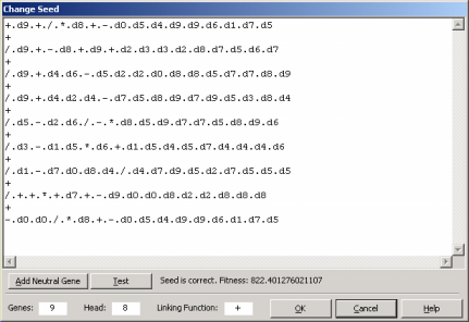
Here, by pressing the Add Neutral Gene button, you will see a neutral gene being added to your model. By doing this, you are giving the learning algorithm more room to play and, hopefully, a better, more complex program will evolve.
Neutral genes can also be introduced automatically by APS 3.0 using the Complexity Increase
Engine.
Complexity Increase Engine
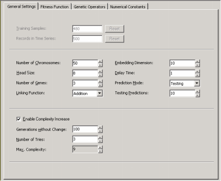
Automatic Problem Solver 3.0 also allows you to introduce neutral genes automatically by activating the Complexity Increase
Engine in the Settings Panel -> General Settings Tab.
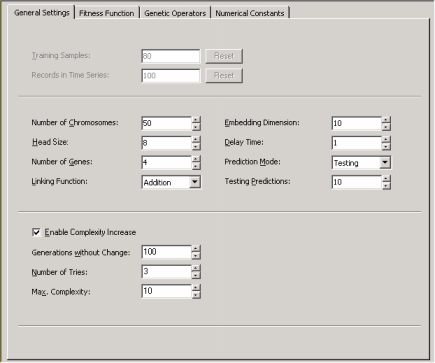
Whenever you are using the Complexity Increase Engine of APS 3.0, you must fill the Generations Without Change box to set the period of time you think acceptable for evolution to occur without improvement in best fitness, after which
a mass extinction or a neutral gene (an extra term) is automatically added to your model; the Number of Tries box corresponds to the
number of consecutive evolutionary epochs (defined by the parameter
Generations Without Change) you will allow before a neutral gene is
introduced in all evolving models; in the Max. Complexity box you write the maximum number of terms (genes) you’ll allow in your model and no other terms will be introduced beyond this threshold.
The Complexity Increase Engine of APS 3.0 might be a very powerful modeling tool, especially for time series prediction models where good models could take longer to come by, but you must be careful not to create excessively complex models as a greater complexity does not necessarily imply a greater
predictive power.
Visualizing Models as Parse Trees
Automatic Problem Solver 3.0 comes equipped with a parse tree maker that automatically converts your models into diagram representations or
parse trees.
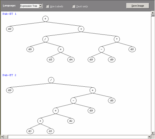
Indeed, the models evolved by APS in its native Karva language can be automatically parsed into visually appealing expression trees, allowing a quicker and more complete understanding of their mathematical intricacies.
Generating Code Automatically Using APS Built-in Grammars
Automatic Problem Solver 3.0 offers a total of eight built-in grammars so that the models evolved by APS in its native
Karva language can be automatically translated into the most commonly used programming languages (C, C++, C#, Visual Basic, VB.Net, Java, Java Script,
and Fortran). This code can then be used in other applications.
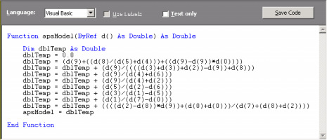
Generating Code Automatically Using User Defined Grammars
Automatic Problem Solver 3.0 allows the design of User Defined Grammars so that the models evolved by APS in its native
Karva language can be automatically translated into the programming language of your choice if you happen to prefer a programming language not already covered by the
eight built-in grammars of APS 3.0 (C, C++, C#, Visual Basic, VB.Net, Java, Java Script,
and Fortran).
As an illustration, the C++ grammar of APS 3.0 is shown in here.
Other grammars may be easily created using this or other APS built-in grammar as reference.
Making Predictions
The algorithms of APS 3.0 used for Time Series Prediction allow not only the evolution of models but also to use these models to make predictions.
APS 3.0 allows you to make two kinds of predictions: one for testing past known events and another for making predictions about the future. In both cases, though, predictions are made recursively, by evaluating the forecast at
t +1, then using it to forecast t+2, and so on.
You must choose either one of these methods while loading your time series data, as this imposes some constraints on the restructuring of the time series for training.
Namely,
n testing records (the n last ones) are saved for
testing and sometimes a small number of records from the top must be
deleted. However, you can also change these parameters later in the
APS modeling environment.
Thus, the first type – Testing Mode – can be used for research or pre-evaluation purposes, as it allows you to test the forecasting capabilities of your model on a set of test observations.
The second type – Prediction Mode – is used obviously to predict unknown behavior, and APS 3.0 allows you to venture into the future as far as you see fit, by setting the number of predictions you want to make and then click the Predict button.
Like for the Testing Mode, the predictions can be plotted together
with the Target and the Model output or be shown separately in a
different plot.
|