Before evolving a model with APS 3.0 you must first load
and transform the input data for the learning algorithm.
To Load Input Data for Modeling
- Click the Run menu and then choose New.
The New Run wizard appears. You must give a name to your new run file (the default filename extension of APS 3.0 run files is .gep) and choose the problem category.
- Go to the Data Source window by clicking the Next button.
For time series prediction problems only text files can be used
for input.
- Then go to the Data Files dialog box by clicking the Next button.
Choose the path for the time series by browsing the Open dialog box.
- Then go to the Time Series Transformation dialog box by clicking the Next button.
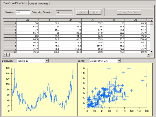
Set the appropriate Embedding Dimension and Delay Time for transforming the time series. Then, depending on whether you wish to make predictions about the future or test the predictive power of the evolved models on known behavior, choose either Testing or Prediction.
- Click the Next button to load and transform the time series.
The Testing Datasets dialog box appears and there you can monitor both the original and transformed time series.
- Click the Next button and then Finish to save your new run file.
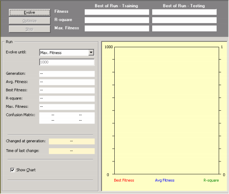
The Save As dialog box appears and after choosing the directory where you want your new run file to be saved, the Automatic Problem Solver 3.0 modeling environment appears.
Then you just have to click the Evolve button to create a model as APS 3.0 automatically chooses, from a gallery of templates, default settings that will enable you to evolve a model immediately.
In time series modeling, be it performed by learning algorithms or conventional statistical methods, it is extremely important the way one chooses to transform the time series before embarking on a complex, usually time consuming modeling process.
First of all, there is the size of the time series to consider and how you choose to transform it, that is, which values will be chosen for the
Embedding Dimension and the Delay Time, because all these factors together will determine the number of
Training Samples actually used for modeling.
The time series transforming engine of APS 3.0 is operational every time you create a new run or every time you change either the
Embedding Dimension or the Delay Time, the Prediction Mode or the
number of Testing Predictions during a
run in the General Settings Tab.
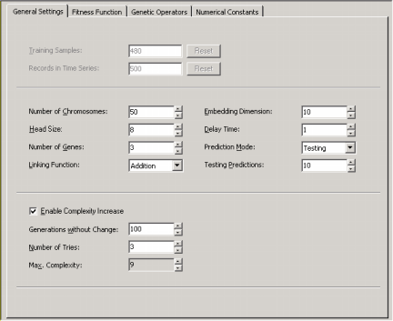
In practice, the embedding dimension corresponds to the number of independent variables or terminals after your time series has been transformed and, therefore, will have a strong impact on the complexity of the problem.
The delay time t determines how data are processed, that is, continuously if
t = 1 or at t
intervals.
These two parameters, together with the size of the time series and
the prediction mode, will determine the final number of training samples after the transformation of the time series.
The data are then ready for evolving prediction models with them and can be visualized in the
Data
Panel before evolving a new model.
And, as for Function Finding or Classification problems, it is important to
choose a reasonable number of samples for training: an excessively large number of samples will slow the modeling process unnecessarily. A good rule of thumb consists of using about 8-10 samples for each independent variable in your training data. For instance, for a time series with 100 observations, an embedding dimension of 10 and a delay time of one, will result in a training set with 90 samples which consists of an extremely well balanced training set.
|