The learning algorithm APS 3.0 uses for
classification, classifies your input data into two classes: class "0" and class "1". Obviously, the dependent variable in your training and testing sets
can only have two distinct values: 0 or 1.
APS 3.0 classifies the value returned by the evolved model as
"1" or "0" using the 0/1 Rounding Threshold. If the value returned by the evolved model is equal to or greater than the rounding threshold, then the record is classified as
"1", "0" otherwise.
Classification problems with more than two classes are also easily solved with APS 3.0. When you are classifying data into more than two classes, say,
n distinct classes, you must decompose your problem into n separate 0/1 classification tasks as follows:
C1 versus Not C1
C2 versus Not C2
...
Cn versus Not Cn
Then evolve n different models separately and combine the different models to make the final
classification model.
But before evolving a model with APS 3.0 you must first load the input data for the learning algorithm.
To Load Input Data for Modeling
- Click the Run menu and then choose New.
The New Run wizard appears. You must give a name to your new run file (the default filename extension of APS 3.0 run files is .gep) and choose the problem category.
- Go to the Data Source window by clicking the Next button and choose the kind of source file.
- Then go to the Data Files dialog box by clicking the Next button.
Choose the path for the training set by browsing the Open dialog box. Do the same for the testing set if you wish to evaluate the generalizing abilities of your model.
- Click the Next button to load the input data.
The Testing Datasets dialog box appears only if your datasets
are correct as APS automatically screens your datasets for
nominal, missing or incorrect values and prompts you to correct
them.
- Click the Next button and then Finish to save your new run file.
The Save As dialog box appears and after choosing the directory where you want your new run file to be saved, the Automatic Problem Solver 3.0 modeling environment appears.
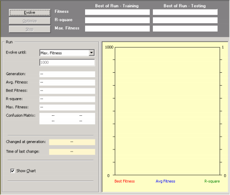
Then you just have to click the Evolve button to create a model as APS 3.0 automatically chooses, from a gallery of templates, default settings that will enable you to evolve a model immediately.
In data mining, be it performed by learning algorithms or conventional statistical methods, it really pays to take a good look at your data before embarking on a complex, usually time consuming modeling process. It's true that evolutionary algorithms are particularly well equipped to deal with noisy data, but the better the data you feed them the better the models they produce.
Automatic Problem Solver helps you find missing and invalid (usually nominal) values in your data sets and prompts you to fix them before they are used for modeling. But the preparation of a well balanced data set should be done before loading the data into APS, and we recommend you to particularly take care of the following:
- Avoid using duplicated samples for they can bias the modeling process considerably.
- Choose a well balanced data set.
- Choose a reasonable number of samples for training.
An excessively large data set will slow the modeling process unnecessarily. If you have access to huge data bases it’s good practice to use the surplus samples for testing instead. A good rule of thumb consists of using about 8-10 samples for each independent variable in your training data.
- Check your data sets carefully for inaccurate values. Typographical or measurement errors generally cause outliers that can be detected by graphing one variable at a time.
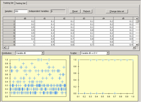
Data cleaning is a time-consuming and labor-intensive procedure, but one that is absolutely necessary for successful modeling. The
graphical visualization tools of APS 3.0 make it easy to identify outliers, which may well represent errors in the data files. After loading your data into APS, in the
Data Panel you can visualize the distribution of values for each variable and also plot each independent variable against the dependent variable.
|